Have you encountered a data set with more than 1000 features? More than 50,000? I have encountered. Dimensionality reduction is a very challenging task, especially when you don't know where to start. Having so many variables is a blessing-the larger the amount of data, the more credible the analysis results are; it is also a curse-you will really feel at a loss and have nowhere to start.
Faced with so many characteristics, it is obviously not feasible to analyze each variable at the micro level, because it will take at least a few days or even months, and the time cost behind this is difficult to estimate. To this end, we need a better way to deal with high-dimensional data, such as the dimensionality reduction introduced in this article: a method that can reduce the number of features in the data set while avoiding losing too much information and maintaining/improving model performance.

What is dimensionality reduction?
Every day, we generate a lot of data. In fact, about 90% of the data in the world is generated in the past 3 to 4 years. This is an incredible reality. If you don’t believe me, here are a few examples of collected data:
Facebook will collect data about what you like, share, post, and visit, such as which restaurant you like.
Various applications in smartphones collect a lot of personal information about you, such as your location.
Taobao collects data about what you purchase, view, and click on its website.
The casino will track every move of every customer.
As data is generated and the amount of data collected continues to increase, it becomes more and more difficult to visualize and draw inference diagrams. Under normal circumstances, we often draw charts to visualize data. For example, suppose we have two variables at hand, one age and one height. We can draw a scatter chart or a line chart to easily reflect the relationship between them.
The following figure is a simple example:
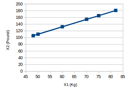
The unit of the abscissa X1 is "kilogram", and the unit of the ordinate X2 is "pound". It can be found that although there are two variables, the information they convey is the same, that is, the weight of the object. So we only need to choose one of them to retain the original meaning. After compressing the 2-dimensional data to 1-dimensional (Y1), the above picture becomes:

Similarly, we can transform the data from the original p-dimension into a series of k-dimension subsets (k
Why dimensionality reduction?
The following is the use of dimensionality reduction in the data set:
As data dimensions continue to decrease, the space required for data storage will also decrease.
Low-dimensional data helps reduce calculation/training time.
Some algorithms tend to perform poorly on high-dimensional data, and dimensionality reduction can improve the usability of the algorithm.
Dimensionality reduction can solve the problem of multicollinearity by removing redundant features. For example, we have two variables: "time spent on the treadmill over a period of time" and "calorie consumption". These two variables are highly correlated. The longer you spend on the treadmill, the more calories you burn. Therefore, it does not make much sense to store these two data at the same time, just one is enough.
Dimensionality reduction helps data visualization. As mentioned earlier, if the dimensionality of the data is very high, visualization will become quite difficult, and it is very simple to graph the two-dimensional and three-dimensional data.
Data set 1: Big Mart Sales III
Overview of dimensionality reduction technologies
There are two main ways to reduce the data dimension:
Only the most relevant variables (feature selection) in the original data set are retained.
Look for a new set of smaller variables, where each variable is a combination of input variables and contains basically the same information as the input variables (dimensionality reduction).
1. Missing Value Ratio
Assuming you have a data set, what will you do in the first step? Before building a model, exploratory analysis of the data is essential. But in the process of browsing the data, we sometimes find that it contains a lot of missing values. If there are few missing values, we can fill in the missing values ​​or delete the variable directly; if there are too many missing values, what will you do?
When the proportion of missing values ​​in the data set is too high, I generally choose to delete this variable directly because it contains too little information. But the specific deletion or deletion depends on the situation. We can set a threshold. If the proportion of missing values ​​is higher than the threshold, delete the column where it is located. The higher the threshold, the more aggressive the dimensionality reduction method.
The following is the specific code:
# Import the required libraries
import pandas as pd
import numpy as np
import matplotlib.pyplot as plt
Download Data:
# Read data
train=pd.read_csv("Train_UWu5bXk.csv")
[Note]: The path of the file should be added when reading the data.
Use .isnull().sum() to check the proportion of missing values ​​in each variable:
train.isnull().sum()/len(train)*100
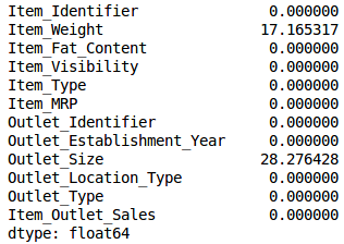
As shown in the table above, there are few missing values. We set the threshold to 20%:
# Save missing values ​​in variables
a = train.isnull().sum()/len(train)*100
# Save column names
variables = train.columns
variable = []
for i in range(0,12):
if a[i]
variable.append(variables[i])
2. Low Variance Filter
If we have a data set in which the values ​​of a certain column are basically the same, that is, its variance is very low, does this variable still have value? Consistent with the idea of ​​the previous method, we usually think that the amount of information carried by the low variance variable is also very small, so it can be deleted directly.
Putting it into practice is to calculate the variance of all variables first, and then delete the smallest ones. One thing to note is: the variance is related to the data range, so the data needs to be normalized before using this method.
In the example, we first estimate the missing value:
train['Item_Weight'].fillna(train['Item_Weight'].median, inplace=True)
train['Outlet_Size'].fillna(train['Outlet_Size'].mode()[0], inplace=True)
Check whether missing values ​​have been filled in:
train.isnull().sum()/len(train)*100
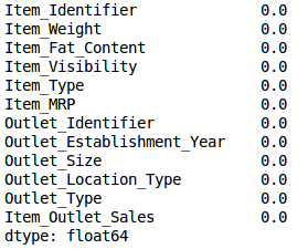
Then calculate the variance of all numerical variables:
train.var()

As shown in the figure above, the variance of Item_Visibility is very small compared with other variables, so it can be deleted directly.
umeric = train[['Item_Weight','Item_Visibility','Item_MRP','Outlet_Establishment_Year']]
var = numeric.var()
numeric = numeric.columns
variable = []
for i in range(0,len(var)):
ifvar[i]>=10: # Set the threshold to 10%
variable.append(numeric[i+1])
The above code helps us list all variables with variance greater than 10.
3. High Correlation filter
If two variables are highly correlated, it means that they have similar trends and may carry similar information. In the same way, the existence of such variables will reduce the performance of some models (such as linear and logistic regression models). To solve this problem, we can calculate the correlation between independent numerical variables. If the correlation coefficient exceeds a certain threshold, one of the variables is deleted.
As a general rule, we should keep those variables that show a similar or high correlation with the target variable.
First, delete the dependent variable (ItemOutletSales) and save the remaining variables in a new data column (df).
df=train.drop('Item_Outlet_Sales', 1)
df.corr()

As shown in the above table, there are no highly correlated variables in the sample data set, but under normal circumstances, if the correlation between a pair of variables is greater than 0.5-0.6, then you should consider whether to delete a column.
4. Random Forest
Random forest is a widely used feature selection algorithm, which automatically calculates the importance of each feature, so there is no need for separate programming. This helps us choose a smaller subset of features.
Before starting the dimensionality reduction, we first convert the data into a digital format, because the random forest only accepts digital input. At the same time, although the variable ID is a number, it is not important at present, so it can be deleted.
from sklearn.ensemble importRandomForestRegressor
df=df.drop(['Item_Identifier','Outlet_Identifier'], axis=1)
model = RandomForestRegressor(random_state=1, max_depth=10)
df=pd.get_dummies(df)
model.fit(df,train.Item_Outlet_Sales)
After fitting the model, draw a graph according to the importance of features:
features = df.columns
importances = model.feature_importances_
indices = np.argsort(importances[0:9]) # top 10 features
plt.title('Feature Importances')
plt.barh(range(len(indices)), importances[indices], color='b', align='center')
plt.yticks(range(len(indices)), [features[i] for i in indices])
plt.xlabel('Relative Importance')
plt.show()
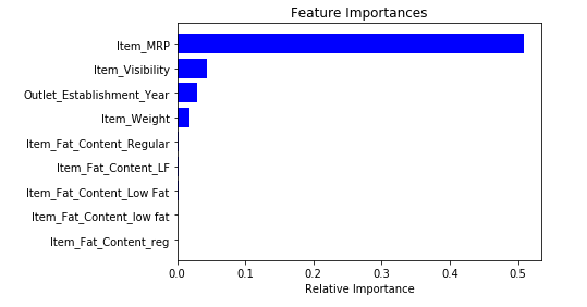
Based on the above figure, we can manually select the topmost feature to reduce the dimensionality in the data set. If you are using sklearn, you can directly use SelectFromModel, which selects features based on the importance of weights.
from sklearn.feature_selection importSelectFromModel
feature = SelectFromModel(model)
Fit = feature.fit_transform(df, train.Item_Outlet_Sales)
5. Backward Feature Elimination
The following are the main steps of reverse feature elimination:
First get all n variables in the data set, and then use them to train a model.
Calculate the performance of the model.
Calculate the performance of the model after deleting each variable (n times), that is, we remove one variable each time and train the model with the remaining n-1 variables.
Determine the variable that has the least impact on the performance of the model and delete it.
Repeat this process until you can no longer delete any variables.
This method can be used when constructing linear regression or logistic regression models.
from sklearn.linear_model importLinearRegression
from sklearn.feature_selection import RFE
from sklearn import datasets
lreg = LinearRegression()
rfe = RFE(lreg, 10)
rfe = rfe.fit_transform(df, train.Item_Outlet_Sales)
We need to specify the algorithm and the number of features to be selected, and then return the variable list of the reverse feature elimination output. In addition, rfe.ranking_ can be used to check variable ranking.
6. Forward Feature Selection
Forward feature selection is actually the reverse process of reverse feature elimination, that is, finding the best features that can improve the performance of the model, rather than deleting weak-influencing features. The idea behind it is as follows:
Choose a feature, train the model n times with each feature, and get n models.
The variable with the best model performance is selected as the initial variable.
Each time you add a variable to continue training, repeat the previous process, and finally retain the variable with the largest performance improvement.
Keep adding and filtering until the model performance no longer improves significantly.
from sklearn.feature_selection import f_regression
ffs = f_regression(df,train.Item_Outlet_Sales)
The above code will return an array, which includes the variable F value and the p value corresponding to each F. Here, we select variables with F values ​​greater than 10:
variable = []
for i in range(0,len(df.columns)-1):
if ffs[0][i] >=10:
variable.append(df.columns[i])
[Note]: Forward feature selection and reverse feature elimination are time-consuming and computationally expensive, so they are only suitable for data sets with fewer input variables.
So far, the six methods we have introduced can well solve the example shopping mall sales forecasting problem, because this data set itself does not have many input variables. In the following, in order to show the dimensionality reduction method of a multivariate data set, we will change the data set to Fashion MNIST, which has 70,000 images in total, including 60,000 images in the training set and 10,000 images in the test set. Our goal is to train a model that can classify various clothing accessories.
Data set 2: Fashion MNIST
7. Factor Analysis
Factor analysis is a common statistical method, which can extract common factors from multiple variables and obtain the optimal solution. Suppose we have two variables: income and education. They may be highly correlated because, overall, people with higher education generally have higher incomes, and vice versa. So they may have a potential commonality factor, such as "ability."
In factor analysis, we group variables according to their correlations, that is, all variables within a specific group are highly correlated, and variables between groups are less correlated. We call each group a factor, which is a combination of multiple variables. Compared with the variables in the original data set, these factors are fewer in number, but the information they carry is basically the same.
import pandas as pd
import numpy as np
from glob import glob
import cv2
images = [cv2.imread(file) for file in glob('train/*.png')]
[Note]: You must replace the path in the glob function with the path of the train folder.
Now we first convert these images to numpy array format in order to perform mathematical operations and draw images.
images = np.array(images)
images.shape
Returns: (60000, 28, 28, 3)
As shown above, this is a three-dimensional array, but our goal is to convert it into one-dimensional, because subsequent only accept one-dimensional input. So we have to flatten the image:
image = []
for i in range(0,60000):
img = images[i].flatten()
image.append(img)
image = np.array(image)
Create a data frame that contains the pixel value of each pixel and their corresponding labels:
train = pd.read_csv("train.csv") # Give the complete path of your train.csv file
feat_cols = ['pixel'+str(i) for i in range(image.shape[1])]
df = pd.DataFrame(image,columns=feat_cols)
df['label'] = train['label']
Use factor analysis to decompose the data set:
from sklearn.decomposition importFactorAnalysis
FA = FactorAnalysis(n_components = 3).fit_transform(df[feat_cols].values)
Here, n_components will determine the number of factors in the converted data. After the conversion is complete, visualize the results:
%matplotlib inline
import matplotlib.pyplot as plt
plt.figure(figsize=(12,8))
plt.title('Factor Analysis Components')
plt.scatter(FA[:,0], FA[:,1])
plt.scatter(FA[:,1], FA[:,2])
plt.scatter(FA[:,2],FA[:,0])
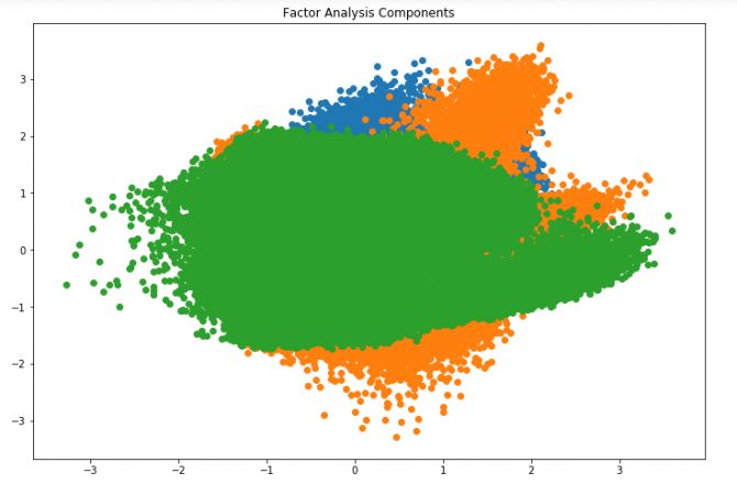
In the above figure, the x-axis and y-axis represent the value of the decomposition factor. Although the common factor is latent and difficult to observe, we have successfully reduced the dimensionality.
8. Principal component analysis (PCA)
If factor analysis assumes that there are a series of latent factors that can reflect the information carried by the variables, then PCA is to transform the original n-dimensional data set into a new data set called the principal component through orthogonal transformation, that is, from the existing Extract a new set of variables from a large number of variables. Here are some key points about PCA:
The principal component is a linear combination of the original variables.
The first principal component has the largest variance value.
The second principal component attempts to explain the remaining variance in the data set, and is not correlated with the first principal component (orthogonal).
The third principal component tries to explain the unexplained variance such as the first two principal components.
Before further dimensionality reduction, we first randomly draw some graphs in the data set:
rndperm = np.random.permutation(df.shape[0])
plt.gray()
fig = plt.figure(figsize=(20,10))
for i in range(0,15):
ax = fig.add_subplot(3,5,i+1)
ax.matshow(df.loc[rndperm[i],feat_cols].values.reshape((28,28*3)).astype(float))
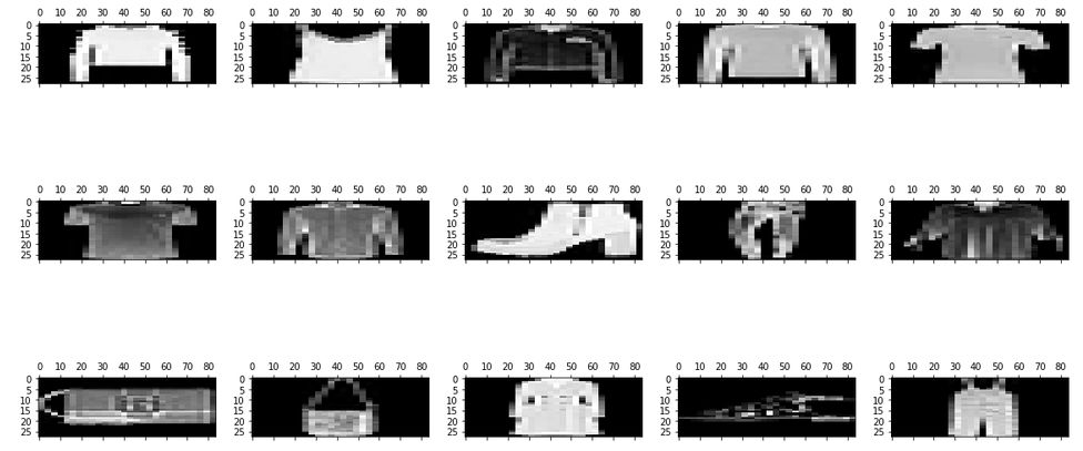
To achieve PCA:
from sklearn.decomposition import PCA
pca = PCA(n_components=4)
pca_result = pca.fit_transform(df[feat_cols].values)
Among them, n_components will determine the principal components in the converted data. Next, let's take a look at how much variance these four principal components explain:
plt.plot(range(4), pca.explained_variance_ratio_)
plt.plot(range(4), np.cumsum(pca.explained_variance_ratio_))
plt.title("Component-wise and Cumulative Explained Variance")
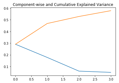
In the figure above, the blue line represents the variance explained by the components, and the orange line represents the cumulative explained variance. We only used four components to explain about 60% of the variance in the data set.
9. Independent component analysis (ICA)
Independent component analysis (ICA) is based on information theory and is one of the most widely used dimensionality reduction techniques. The main difference between PCA and ICA is that PCA looks for unrelated factors, while ICA looks for independent factors.
If two variables are not related, there is no linear relationship between them. If they are independent, they do not depend on other variables. For example, a person’s age has nothing to do with what he ate/watched on TV.
The algorithm assumes that the given variable is a linear mixture of unknown latent variables. It also assumes that these latent variables are independent of each other, that is, they do not depend on other variables, so they are called independent components of the observed data.
The figure below is an intuitive comparison between ICA and PCA:
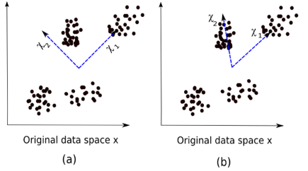
(a) PCA, (b) ICA
The equation for PCA is x = Wχ.
Here,
x is the observation
W is the mixed matrix
χ is the source or independent component
Now we must find a non-mixing matrix to make the components as independent as possible. The most commonly used method to test component independence is non-Gaussian:
According to the Central Limit Theorem (Central Limit Theorem), a mixture of multiple independent random variables will tend to be normally distributed (Gaussian distribution).
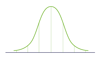
Therefore, we can find the component that maximizes kurtosis among all independent components.
Once the kurtosis is maximized, the entire distribution will show a non-Gaussian distribution, and we can also get independent components.
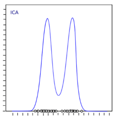
Implement ICA in Python:
from sklearn.decomposition importFastICA
ICA = FastICA(n_components=3, random_state=12)
X=ICA.fit_transform(df[feat_cols].values)
10. IOSMAP
Code:
from sklearn import manifold
trans_data = manifold.Isomap(n_neighbors=5, n_components=3, n_jobs=-1).fit_transform(df[feat_cols][:6000].values)
Parameters used:
n_neighbors: Determine the number of adjacent points for each point
n_components: determines the number of coordinates of the manifold
n_jobs = -1: Use all available CPU cores
Visualization:
plt.figure(figsize=(12,8))
plt.title('Decomposition using ISOMAP')
plt.scatter(trans_data[:,0], trans_data[:,1])
plt.scatter(trans_data[:,1], trans_data[:,2])
plt.scatter(trans_data[:,2], trans_data[:,0])
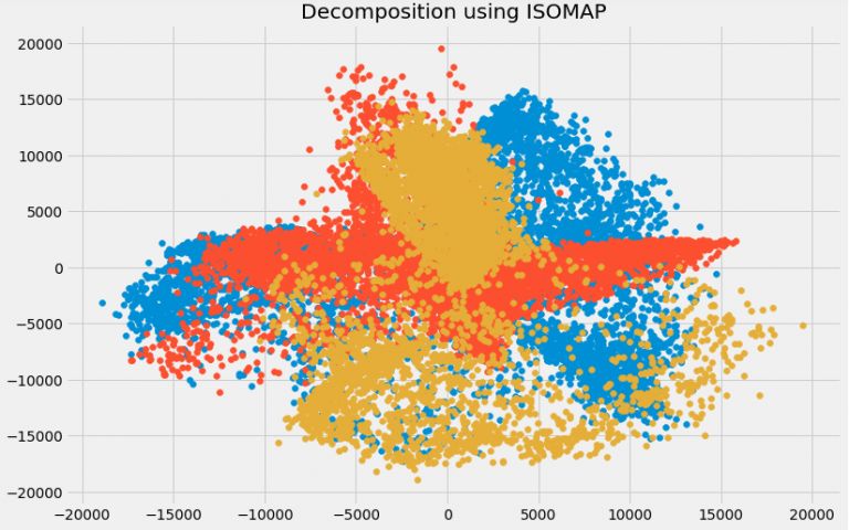
11. t-SNE
Code:
from sklearn.manifold import TSNE
tsne = TSNE(n_components=3, n_iter=300).fit_transform(df[feat_cols][:6000].values)
Visualization:
plt.figure(figsize=(12,8))
plt.title('t-SNE components')
plt.scatter(tsne[:,0], tsne[:,1])
plt.scatter(tsne[:,1], tsne[:,2])
plt.scatter(tsne[:,2], tsne[:,0])
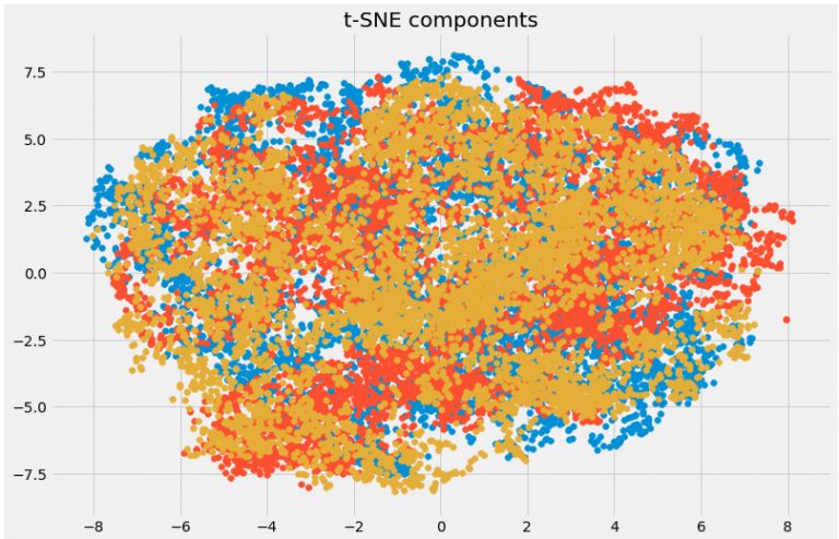
12. UMAP
Code:
import umap
umap_data = umap.UMAP(n_neighbors=5, min_dist=0.3, n_components=3).fit_transform(df[feat_cols][:6000].values)
Here,
n_neighbors: Determine the number of neighboring points.
min_dist: Controls the tightness of the embedding. A larger value can ensure a more uniform distribution of embedding points.
Visualization:
plt.figure(figsize=(12,8))
plt.title('Decomposition using UMAP')
plt.scatter(umap_data[:,0], umap_data[:,1])
plt.scatter(umap_data[:,1], umap_data[:,2])
plt.scatter(umap_data[:,2], umap_data[:,0])
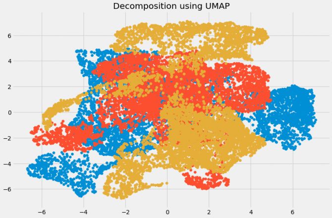
to sum up
So far, we have introduced 12 dimensionality reduction methods. Considering the length, we did not introduce the principles of the latter three methods in detail. Interested readers can find the information, because any one of them is enough to write a special article. Long introduction. This section will summarize these 12 methods and briefly introduce their advantages and disadvantages.
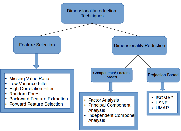
Missing value ratio: If there are too many missing values ​​in the data set, we can use this method to reduce the number of variables.
Low variance filtering: This method can identify and delete constant variables from the data set. Variables with small variance have little effect on the target variable, so you can safely delete it.
High correlation filtering: A pair of variables with high correlation will increase the multicollinearity in the data set, so it is necessary to delete one of them in this way.
Random Forest: This is one of the most commonly used dimensionality reduction methods, it will clearly calculate the importance of each feature in the data set.
Forward feature selection and reverse feature elimination: These two methods are time-consuming and computationally expensive, so they are only suitable for data sets with fewer input variables.
Factor analysis: This method is suitable for situations where there are highly correlated variable sets in the data set.
PCA: This is one of the most widely used techniques for processing linear data.
ICA: We can use ICA to convert data into independent components and use fewer components to describe the data.
ISOMAP: suitable for non-linear data processing.
t-SNE: It is also suitable for non-linear data processing. Compared with the previous method, the visualization of this method is more direct.
UMAP: Suitable for high-dimensional data. Compared with t-SNE, this method is faster.
TSVAPE, we bring in the best vape pod systems, pod kits for wholesaler and advanced vapers.Pod systems and pod kits are reshaping the trends of vaping industry to brilliance!
We provide products such as RELX,YOOZ,SNOWPLUS,FLOW,FOLI,LANA
Please contact us. If you are interested, we guarantee 100% original products at reasonable prices.


Vape Pods And Kits,Compact Vape Pod Kits,Pod Vape Kits,E Cigarette Pods And Kits
TSVAPE Wholesale/OEM/ODM , https://www.tsecigarette.com